Beam Search

Generate text by exploring multiple paths at once, keeping the most promising candidates at each step.

You will need

• a completed model from an earlier lesson
• pen and paper for each “beam” (or a whiteboard divided into columns)
• dice for sampling (or use greedy selection)
• multiple people to track different beams (works best as a group activity)

Your goal

Generate text using beam search with beam width 2 or 3. Compare the result to standard single-path generation. Stretch goal: try different beam widths and see how results change.

Key idea

Standard generation picks one word at a time and commits to it. Beam search keeps multiple candidates alive, only choosing the final output after seeing how each path develops. This often produces more coherent text.

Algorithm

Setup

1. Choose a beam width (start with 2 or 3—this is how many paths you track).
2. Assign one person (or paper column) to each beam.
3. Agree on a scoring method: sum of counts along the path, or product of probabilities.

Generation

1. Start: all beams begin with the same starting word.

2. Expand: for each beam, find all possible next words from the current word’s row.

3. Score: calculate the score for each possible continuation (current path score + new word’s count, or current score × new word’s probability).

4. Prune: across all beams and all their expansions, keep only the top k paths (where k is your beam width). Some beams may die; others may branch.

5. Repeat: continue until all surviving beams reach a stopping point (.) or target length.

6. Select: choose the highest-scoring complete path as your output.

Example

Model: trained on “See Spot run. See Spot jump.”

Beam width: 2

Step 1 (start): both beams have “see” (score: 0)

Step 2 (expand from “see”):

• “see → spot” is the only option (count: 2)
• Both beams: “see spot” (score: 2)

Step 3 (expand from “spot”):

• “spot → run” (count: 1)
• “spot → jump” (count: 1)
• Beam 1: “see spot run” (score: 3)
• Beam 2: “see spot jump” (score: 3)

Step 4 (expand from “run” and “jump”):

• “run → .” (count: 1) → Beam 1: “see spot run.” (score: 4)
• “jump → .” (count: 1) → Beam 2: “see spot jump.” (score: 4)

Final: tied scores, so either output works. In practice, you’d pick one arbitrarily or continue generating.

Tracking beams in practice

With people: each person holds a piece of paper showing their current path and score. After each expansion step, everyone announces their candidates. The group collectively picks which paths survive.

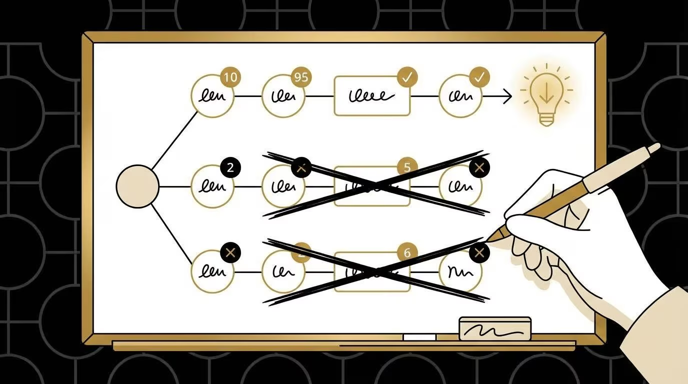
With a whiteboard: draw columns for each beam. Write paths vertically, crossing out eliminated paths and continuing survivors.

With cards: write each candidate path on an index card. Spread them out, score them, and physically remove the losers.

Instructor notes

Discussion questions

• how does beam width affect output quality?
• what happens with beam width 1? (it’s just greedy search)
• what happens with very large beam width? (approaches exhaustive search)
• when would beam search produce different results than random sampling?
• can a path that looks bad early become the best path later?

Comparing methods

Run the same starting word through three methods:

1. Random sampling (dice rolls)
2. Greedy (always pick highest count)
3. Beam search (width 2–3)

Compare the outputs. Beam search often finds a middle ground—more coherent than random, less repetitive than greedy.

Computational trade-offs

Discuss with students:

• beam width 1 = 1 path to track (fast, simple)
• beam width 10 = 10 paths to track (slower, but explores more options)
• beam width 1000 = impractical by hand, but computers can do it

This illustrates why AI researchers tune beam width: it’s a trade-off between computation time and output quality.

Connection to current LLMs

Beam search is a classic decoding strategy used in many language tasks:

• machine translation: beam search finds fluent translations by exploring multiple word orders
• speech recognition: keeps multiple interpretations alive until context disambiguates
• code generation: explores different syntactic structures before committing
• trade-offs: beam search guarantees finding high-probability sequences but can produce “boring” text; sampling adds creativity but risks incoherence

The key insight: generation is a search problem. Standard sampling explores one random path; greedy search explores one “obvious” path; beam search explores multiple promising paths. Your classroom beams demonstrate this directly—by tracking several candidates, you can compare outcomes that single-path methods would never see.

Modern LLMs often combine strategies: use beam search for factual tasks where accuracy matters, sampling for creative tasks where variety matters, and hybrid approaches that sample within beams for balanced results.